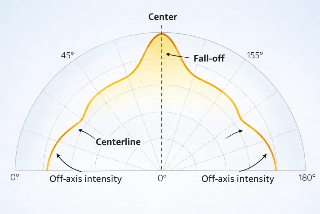
In lighting contexts, a “COB LED strip emission graph” is usually a distribution graphic (often a polar curve) showing how intensity changes with angle. Some searches use “emission graph” to mean a spectral (SPD) graph for color quality, so always check the axes.
Distribution/polar curve = how the light spreads by angle (helps with profiles, diffusers, and sightlines).
Spectral/SPD graph = what colors the light contains (not beam spread).
Quick read (3 steps):
Confirm the axes: angle-based (distribution) vs wavelength-based (spectrum).
On a polar curve, check fall-off away from center and any strong off-axis intensity.
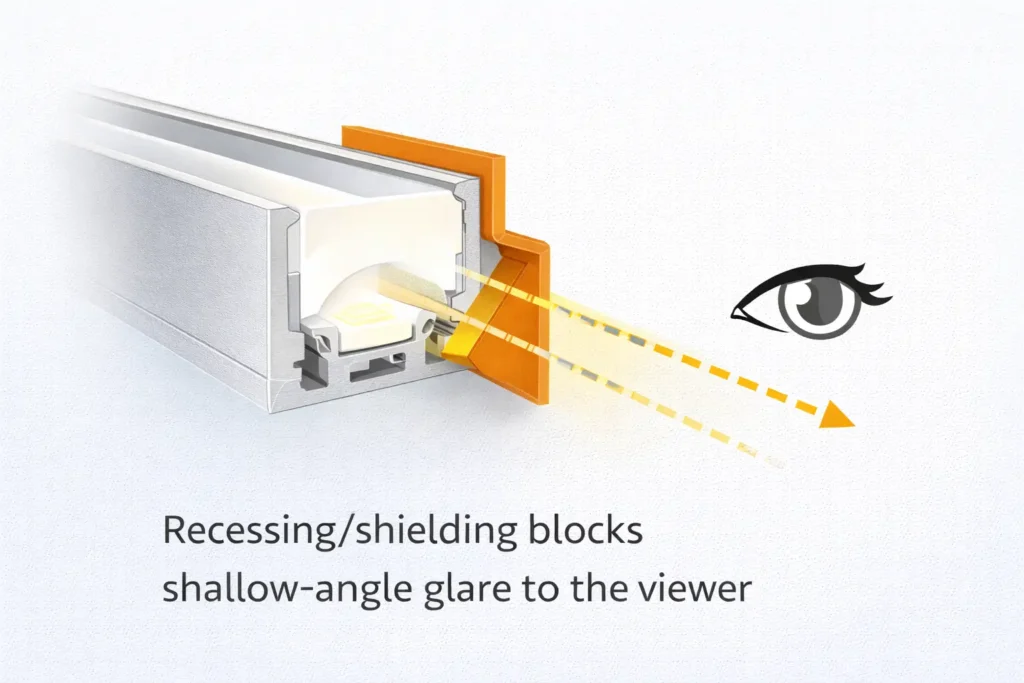
Map to install: off-axis intensity often needs recessing/shielding to stay comfortable.
Boundary conditions:
Many “graphs” are schematic; treat them as directional unless tied to a measured photometric file/report for the exact SKU.
Installed appearance is system-dependent.
What a COB LED Strip Emission Graph Shows (and What It Doesn’t)
A distribution-style emission graph shows intensity vs angle; it helps you compare spread and anticipate glare/spill, but it does not guarantee brightness, efficiency, or “dotless” appearance on site.
Tells you: wide vs controlled distribution and off-axis intensity cues.
Helps you choose: diffuser strength, recessing/shielding, and where direct view may be risky.
Doesn’t tell you: total output, electrical limits, or your exact profile/diffuser result.
Boundary conditions:
Treat diagrams as comparison cues unless verified by measured photometry for the exact configuration.
What it tells you (practical uses)
Use distribution information to decide application fit before you commit to a profile system.
Indirect/cove: wider distributions can help even wash.
Direct-view lines: off-axis intensity often becomes glare unless recessed/shielded.
Profile choice: distribution cues suggest how much diffusion and depth you’ll likely need.
Boundary conditions:
Viewing distance and diffuser choice can change the perceived result.
What it doesn’t tell you (common misreads)
The biggest mistake is treating “wide beam” or a nice-looking diagram as proof the installation will be uniform and comfortable.
“Wide = dotless” → dotless depends on diffuser, depth, and sightlines.
“COB = always 180°” → definitions and optics vary; verify the terms used.
“Diagram = measured” → request measured evidence when approval risk is high.
Boundary conditions:
Keep claims tied to the exact SKU/variant used in the project.
Mini Glossary: Emission Graph vs Beam Angle vs Field Angle vs Spectral Graph
These terms describe different views of light; mixing them produces misleading “apples-to-oranges” comparisons.
Term
What it describes
Best used for
Common pitfall
Emission graph (distribution / polar curve)
Intensity vs angle (distribution shape)
Spread, spill/glare tendency, comparing two options
For non-symmetric beams, angles may differ by plane; one number may not describe everything.
Why “180°” claims can be misleading without definitions
“180°” is often used as a shorthand for “very wide,” but without definition and context it can’t be compared reliably across products.
Beam vs field threshold changes the reported angle (50% vs 10%).
Some beams differ by plane (left-right vs up-down).
Diffusers and profiles can change perceived spread and glare in the final install.
Boundary conditions:
Compare like-for-like: same definition, same plane(s), same SKU/variant.
Quick rules for comparing datasheets fairly
A fair comparison starts with definitions and scope, not marketing labels.
Confirm definition for beam/field angle and the plane(s) reported.
Confirm which variants the claim covers (CCT/CRI/voltage/IP and any optical layer).
Confirm whether any “graph” is measured photometry or schematic.
If distribution drives approval, ask for the evidence package for the exact configuration.
Boundary conditions:
Don’t extend one tested configuration to all variants unless scope is confirmed.
How to Read a Polar Emission Graph in 60 Seconds
Read the curve for symmetry, fall-off, and off-axis intensity, then map those cues to blending, spill, and glare risk.
Wider curve → more spill; can help blending but may raise glare risk in direct view.
Strong off-axis intensity → often needs recessing/shielding for comfort.
Fast fall-off → more control; placement becomes more critical for even wash.
Steps (6):
Confirm it’s a polar distribution curve (angle-based), not a spectral chart.
Check symmetry (similar left/right?).
Note how fast intensity falls away from center.
Look for off-axis “shoulders” (high intensity at wide angles).
Compare two curves: more off-axis area usually feels wider.
Add the install assumption: direct view vs diffuser, and likely sightlines.
Boundary conditions:
If the “graph” is just a half-circle icon, treat it as schematic guidance only.
The 60-second read: 6 steps (what to look for first)
Start with symmetry and fall-off; off-axis intensity is the practical glare clue.
Symmetry suggests consistent behavior across the field of view.
Fall-off indicates how quickly the beam softens away from center.
Off-axis intensity predicts spill and potential discomfort in shallow sightlines.
Boundary conditions:
If only one plane is shown, ask whether the other plane differs.
Quick mapping: what “wider” or “strong off-axis” usually means on site
Wide distribution can look smoother on surfaces, but it can also make the source more visible and uncomfortable in direct sightlines.
Wider curve → easier blending behind diffusion; more spill to adjacent surfaces.
Strong off-axis intensity → higher glare risk without recessing/shielding.
Controlled distribution → less spill; gradients can look sharper if placement is wrong.
Boundary conditions:
Reflective finishes and viewing angles can dominate perceived glare.
COB vs SMD Light Distribution: Typical Differences and Selection Implications
COB often looks more continuous, while SMD can look point-like in shallow/direct view—yet distribution behavior is still optics- and installation-dependent.
COB reduces visible dotting in many profiles, but direct view still benefits from diffusion and recessing.
SMD can blend well with the right diffuser/depth and may offer more varied optical designs by family.
Use “COB vs SMD” as a starting point; verify with samples and documentation.
Factor
COB (typical)
SMD (typical)
What to verify
Continuity
More line-like
Points may show in shallow view
Diffuser + profile geometry for sightlines
Distribution shorthand
Often marketed very wide
Often marketed moderate/wide
Definition context; measured vs schematic
Comfort risk
Can be high if visible
Can be high if visible
Off-axis cues + shielding plan
Best-fit
Indirect lines, shallow channels (with caveats)
General installs, controlled designs (by family)
Evidence scope and install assumptions
Boundary conditions:
“Typical” isn’t universal; treat claims as configuration-specific.
What to verify before you standardize COB vs SMD for a project
Standardize the whole system (strip + profile + diffuser + sightlines), not only the strip type.
Define the profile family and diffuser type per application (direct view vs indirect).
Define critical sightlines and viewing distances.
Confirm documentation scope consistency across variants you will purchase.
Boundary conditions:
A single system rarely fits all geometries; plan more than one standard where needed.
Turn Distribution Into Diffuser & Profile Depth Decisions (Dotless as a System Outcome)
Uniform, comfortable linear light comes from matching distribution to diffusion and geometry—COB helps, but dotless still depends on profile depth and sightlines.
More diffusion and more recessing generally improve blending and reduce glare.
Shallow channels and low-diffusion covers are the most common dotless failure mode.
Distribution cues tell you how much shielding you may need for comfort.
Situation
Likely issue
Safer system choice
What to verify
Direct view near eye level
Glare / harsh line
Recess + shielding + diffusion
Mock-up from real sightlines
Shallow profile + clear cover
Hotspots
Higher diffusion or deeper recess
Depth feasibility
Glossy surroundings
Reflections/glare
Shielding + diffusion + aim control
Surface finish + angles
Grazing/accent
Sharp gradients
Controlled distribution + shielding
Desired effect vs comfort
Boundary conditions:
Avoid fixed “mm depth” rules without project context; validate with a sample.
Decision cues: choosing diffusion, recessing, and sightline control
Most problems are solved by three levers: diffusion, recessing, and shielding.
Glare from normal paths → add shielding lips and reduce line-of-sight.
Reflections on glossy surfaces → diffuse more and aim away from occupants.
Boundary conditions:
Mechanical constraints may limit options; plan profiles early.
Why “dotless” can still fail (even with COB)
COB reduces point visibility, but shallow depth, weak diffusion, or shallow viewing angles can still reveal artifacts and glare.
Too shallow → deeper recess or stronger diffusion.
Cover too clear → switch to higher diffusion.
Viewing too close/shallow → add shielding or reposition.
Boundary conditions:
Each fix trades off efficiency vs comfort; choose based on priority.
Uniformity vs Glare: Trade-Offs and Mitigation (Risk Checklist Included)
Wider distributions can improve blending, but they can also increase glare/spill when the source is visible; mitigation is usually diffusion plus sightline control.
Wide + visible → higher glare risk.
Controlled + visible → less spill but gradients can look sharper.
Comfort failures are mostly sightline problems, not strip problems.
Mitigation steps:
Recess the source and add shielding to block shallow-angle view.
Increase diffusion when sparkle/hotspots are visible.
Reposition to light the target surface, not the occupant.
Risk checklist:
Visible from eye level along normal paths?
Glossy surfaces reflecting the source?
Shallow profile with low diffusion?
Comfort-critical space (hospitality/residential/retail)?
Boundary conditions:
Validate with a mock-up when comfort is a top requirement.
Glare-sensitive scenarios (where problems show up first)
Glare shows up fastest when the source is near eye level or reflected by glossy finishes.
Under-cabinet strips visible from standing positions.
Eye-level coves and low ceilings.
Narrow corridors/stairs with shallow, continuous sightlines.
Tile/stone/metal/glass finishes near the source.
Boundary conditions:
Check multiple viewpoints; one “good angle” can hide a problem.
Most mismatches come from a few controllable variables.
Recessing/shielding geometry
Diffusion level
Viewing distance and angle
Surface reflectivity
Alignment/continuity details
Boundary conditions:
Without context, use this as a guide—not a definitive verdict.
Most common fixes (without changing the strip)
Improve results by adjusting diffusion, sightline control, or placement.
Higher diffusion → fewer hotspots/sparkle.
More recess/shielding → less glare.
Repositioning → smoother wash, less spill into eyes.
Boundary conditions:
Some fixes reduce delivered light; confirm requirements.
When to Request an IES File or Photometric Report (Procurement Triggers)
Request an IES file or photometric report when distribution must be documented for approvals, simulation, or glare-sensitive/high-visibility installations.
<
Evidence matters most when the cost of a wrong choice is high (rework/approvals/complaints).
Scope must match the exact SKU/variant and optical configuration.
Boundary conditions:
Evidence availability is model-dependent; confirm scope per SKU/variant.
Request it when… (project scenarios)
Ask for photometric evidence when documentation is part of the decision, not just a “nice to have.”
Approval or tender documents require distribution evidence.
Designers need simulation inputs.
The install is glare-sensitive or highly visible.
You are standardizing across multiple projects.
Boundary conditions:
If the project is low risk and low visibility, a sample/mock-up may be sufficient.
Ask for… (deliverables + scope confirmation)
The fastest way to avoid disputes is to request evidence and scope confirmation for the exact configuration you will install.
File/report format used in your workflow (IES file or equivalent report).
Any stated definition/plane details for angles (if provided).
Installation notes that affect optics (profile/diffuser assumption).
Boundary conditions:
Evidence availability is model-dependent; confirm scope per SKU/variant.
For a documentation check, share the application (direct view/indirect), profile constraints, and critical sightlines so the right strip + diffuser/profile system and supporting documents can be confirmed early.
Datasheet & RFQ Checks Before Ordering (Avoid Mis-Spec)
Use a checklist to confirm definition, scope, and installation context before you accept any distribution or dotless claim.
Lock the exact SKU/variant before copying claims into specs.
Confirm beam/field definitions and whether multiple planes apply.
Confirm measured vs schematic graphs.
Confirm profile/diffuser assumptions and sightline risks.
Confirm compliance/certification scope per model/series when required.
Boundary conditions:
Treat documentation as part of risk control for approval-driven projects.
Quick RFQ addendum template (copy/paste)
A short addendum reduces “assumed” scope and forces definition alignment.
Keep requests tied to the exact installation scenario and variant scope.
Template:
Please confirm the exact LED strip SKU and variant scope (CCT/CRI/voltage/IP and any optical layer).
For any stated beam angle or distribution claim, please confirm the definition threshold used and the reporting plane(s).
If available for this exact configuration, please provide an IES file or photometric report and note the test context.
Intended installation: [direct view / behind diffuser] in [profile/channel type], with [recessing/shielding concept].
Please confirm which compliance/certification documents apply to this specific model/series and variant (if required).
Boundary conditions:
If evidence isn’t available, plan sampling/mock-ups for approval.
Optional: Special / Narrow Beam Strip Options (When Control Matters)
Controlled-beam strip options can help for accent/grazing, but they can increase glare risk and require tighter installation control.
Controlled beams reduce spill; they can also make gradients sharper.
Verification matters: confirm how the optical control is achieved and documented.
Boundary conditions:
Don’t assume universal “angle categories” exist; verify by datasheet and configuration.
Verification questions (avoid over-specifying)
A few questions keep controlled-beam specs realistic and evidence-backed.
Which exact SKU/variant provides the control, and what optical element creates it?
Is measured photometry available for the installed configuration?
What profile/diffuser geometry is assumed?
Any glare-sensitive limitations noted for typical sightlines?
Boundary conditions:
If documentation is limited, treat it as “requires sample validation.”
PREGUNTAS FRECUENTES
These FAQs recap the key definition and decision points needed to read emission graphs and specify COB LED strip systems with fewer surprises.
Focus: distribution/polar graphs for spread and glare decisions (not spectral/SPD graphs).
Keep scope tied to the exact SKU/variant and the intended profile/diffuser system.
Boundary conditions:
If approval risk is high, validate with evidence or a mock-up in the real geometry.
What is a COB LED strip emission graph?
Q: What is a COB LED strip emission graph? A: Usually it’s an angle-based distribution graphic (often a polar curve) showing how intensity changes with viewing angle, which helps you judge spread and glare risk. Some searches use “emission graph” for a spectral (SPD) chart, so check the axes: angle-based is distribution; wavelength-based is spectrum.
How is beam angle defined, and what is field angle?
Q: How is beam angle defined, and what is field angle? A: Beam angle is commonly defined at 50% of peak intensity, while field angle uses a wider 10% threshold. Align terminology with the IES definitions: beam angle y field angle.
How do you read a polar distribution (emission) graph quickly?
Q: How do you read a polar distribution (emission) graph quickly? A: Confirm it’s a polar distribution curve, then check symmetry, fall-off, and off-axis intensity. Wide curves often blend better behind diffusion; strong off-axis intensity usually needs recessing or shielding.
Why can “dotless” still fail in a shallow profile even with COB?
Q: Why can “dotless” still fail in a shallow profile even with COB? A: Dotless is a system outcome: strip + diffuser + profile depth + sightlines. Shallow channels and low-diffusion covers can still show hotspots or create glare; typical fixes are stronger diffusion, more recessing, or shielding.
How do you reduce glare when using wide-distribution COB strips?
Q: How do you reduce glare when using wide-distribution COB strips? A: Reduce direct visibility from critical sightlines by recessing the strip and adding shielding, then adjust diffusion to soften perceived intensity. Reposition the strip to aim light at the target surface, not occupants.
When should you request an IES file or photometric report for a strip project?
Q: When should you request an IES file or photometric report for a strip project? A: Request it for approvals/simulation, glare-sensitive/high-visibility installs, or standardization across projects. Ensure the file/report matches the exact SKU/variant and optical configuration.
Summary & Next Steps (How to Specify with Confidence)
Specify with confidence by following a simple workflow: interpret the distribution correctly, design the profile/diffuser for sightlines, and verify scope/evidence for the exact SKU.
Key takeaways:
Disambiguate “emission graph” (distribution vs spectrum).
Use curves to anticipate spill and glare, not to assume dotless by default.
Align definitions and scope before comparing datasheets.
Treat linear lighting as a system (strip + profile + diffuser + geometry).
Next steps (common triggers):
Custom profiles or tight depths → sample/mock up in the real geometry.
Long, high-visibility runs → verify continuity and sightlines early.
Wet/outdoor areas → confirm configuration and optical impact of sealing.
Certification-sensitive tenders → confirm document scope by model/series.
Boundary conditions:
Avoid one-size-fits-all rules; confirm with project constraints and samples.
For project inquiries or documentation checks, share (1) application type (direct view/indirect), (2) profile depth constraints, (3) critical sightlines, and (4) any approval/certification requirements. You can reference: Elstar LED strip manufacturing.


